Chapter 1: Introduction to Laplace Transforms

Laplace transforms play a crucial role in various fields, particularly in engineering and science, as they convert differential equations into algebraic equations, simplifying their solutions. These transforms are also vital in dynamics and control theory, helping to identify specific parameters that characterize the behavior of complex dynamical systems, such as poles and zeros. This article will cover essential features of Laplace transforms and the techniques for evaluating them.

To initiate our discussion, let's define the one-sided Laplace transform for a function ( f(t) ):

In practical applications, if ( f(t) ) represents a time-dependent function, the variable ( s ) is measured in inverse time units or Hertz, thus serving as a frequency variable. Consequently, ( F(s) ) represents a frequency domain view of ( f(t) ), distinct from the Fourier transform, which analyzes the frequency content within ( f(t) ). It's important to note that ( s ) can take on complex values.

The inverse Laplace transform, also referred to as the Bromwich integral, is defined as:

where

Calculating the inverse Laplace transform typically involves contour integration in the complex plane, often utilizing Cauchy’s integral formula or the Residue theorem. However, in practical scenarios, one can refer to a transform table to find the closest match for the function. Let's examine several examples to clarify these concepts.

Example 1: Laplace Transform of a Constant

We will begin with the Laplace transform of a constant:

The computation of this transform is straightforward:

Example 2: Laplace Transform of a Linear Function

Next, we consider the Laplace transform of a linear function:

This transform can be evaluated using the integration by parts technique:

This approach yields:

The limit in the first term can be evaluated using L'Hôpital's rule, resulting in:

Example 3: Laplace Transform of a Power Function

Let's compute the Laplace transform for a power function:

We utilize integration by parts to reduce the order of ( f(t) ):

The first term is determined through successive applications of L'Hôpital's rule:

From this, we can establish a recursive formula:

Thus, we find:

This leads us to the conclusion that:

Example 4: Laplace Transform of an Exponential Function

Next, we analyze an exponential function:

The Laplace transform is simply:

Using the result from Example 1 regarding the Laplace transform of a constant, we express:

Similarly, we can derive:

Example 5: Laplace Transform of a Combined Function

To evaluate the Laplace transform of:

we integrate our previous examples. We start with a variable transformation concerning the exponential term:

Subsequently, we apply the result from Example 3 to yield:

More generally, we can express:

Example 6: Laplace Transform of a Trigonometric Function

Lastly, we will consider the sine function:

Initially, we express:

We then apply integration by parts:

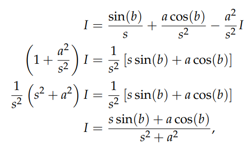
The last term simplifies to ( I ) again, allowing us to rearrange the equation:

Thus, we conclude:

Chapter 2: Additional Resources

To deepen your understanding of Laplace transforms, consider watching the following videos:

The first video titled "Intro to the Laplace Transform & Three Examples" offers an engaging introduction and includes illustrative examples.

The second video, "Q2. Evaluating Laplace Transforms," provides a step-by-step guide on evaluating Laplace transforms, enhancing your comprehension of the topic.